By Péter Sólymos
Linked paper: Lessons learned from comparing spatially explicit models and the Partners in Flight approach to estimate population sizes of boreal birds in Alberta, Canada by P. Sólymos, J.D. Toms, S.M. Matsuoka, S.G. Cumming, N.K.S. Barker, W.E. Thogmartin, D. Stralberg, A.D. Crosby, F.V. Dénes, S. Haché, C.L. Mahon, F.K.A. Schmiegelow, and E.M. Bayne, The Condor: Ornithological Applications.
Population size estimation is experiencing a bit of a renaissance, due in no small part to the recent “three billion birds lost” paper by Rosenberg et al. (2019), which combined trends and population estimates to quantify the number of individual birds that have disappeared over the last 49 years. The tremendous popularity of this paper highlights the notion that people care more about species declines when they can translate trends into numbers of birds.
Ornithologists can use several sources of data to estimate broad-scale bird distribution and migration patterns, such as weather radar maps of bird migration or eBird checklists. But the North American Breeding Bird Survey (BBS) remains the main source of data used to estimate continental landbird population sizes — even though that was not its original purpose. Partners in Flight (PIF) pioneered the development of population estimates for land birds, but they are meant to be very general approximations. By taking advantage of statistical methods that let us control for factors like birds’ singing rates, we can use spatial models to improve population estimates and, as a result, estimates of historical bird losses.
In our recent paper, we looked at how PIF estimates compare to these spatially explicit estimates of bird abundance. This work was a collaborative effort of researchers from the Boreal Avian Modelling (BAM) project, the Canadian Wildlife Service (Environment and Climate Change Canada), and the United States Geological Survey, aimed at developing more accurate status and trend estimates for North American birds. We looked at the following 3 factors that drove the differences between the two estimates.
1. Detection distance
The PIF approach applies adjustments to BBS counts to get population estimates. Efforts to date have been focused on two key factors: detection distance and time adjustments. The maximum detection distance (MDD) represents the largest distance at which a bird can be detected, thus giving a conservative estimate of population size. A more robust approach is to use the concept of effective detection distance based on distance sampling. This measure is used to give an estimate of the area sampled when not all of the birds are counted due to imperfect detection. The difference between maximum and effective detection distance alone can result in significantly higher population estimates and has led to a downward revision of the MDDs used by PIF.
2. Time adjustment
The second factor in the PIF estimator adjusts counts based on timing of surveys relative to when birds are most likely to be counted. Although there is certainly room for improvement (see this paper and blog posts here and here), the time adjustment factor has much less influence on population estimates compared to detection distance.
All of this important work has led to a much-improved recent version of the PIF population estimates database. But it still didn’t deal with the elephant in the room, namely the roadside nature of the BBS data upon which the estimates are based.
3. Roadside effects
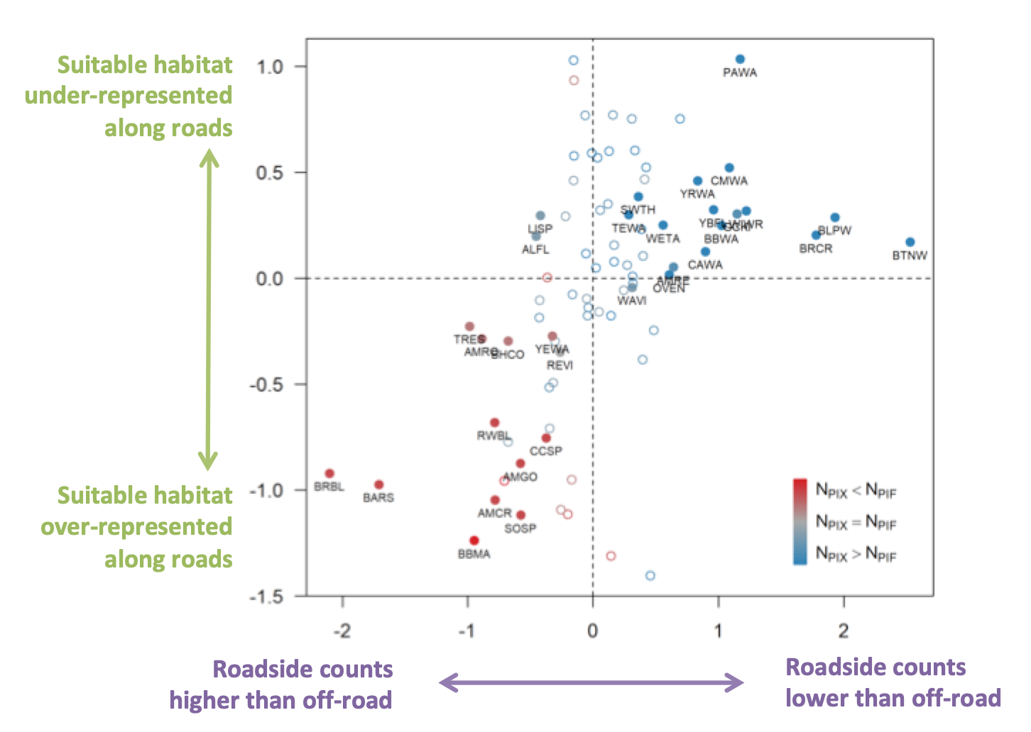
Using roadside data for population estimation has two important consequences. First, the density, behavior, and detectability of species may be different along roads than away from roads. Second, the locations of roads themselves aren’t random, resulting in an unrepresentative sampling of habitats. Our findings show that these two previously unaccounted-for assumptions influence population estimates.
To adjust for this, we developed spatially explicit models for 81 landbird species in northern Alberta, Canada. We combined roadside and off-road data and applied distance-sampling and removal-model based adjustments to account for variable sampling methodology in the data set and survey-level differences in detectability. We then estimated population sizes through spatial prediction — which is why we named the approach “pixel based,” or PIX for short. We then compared PIX and PIF population estimates, and looked at patterns across species.
As expected, we found that time and especially detection distance adjustments explained average differences between the PIF and PIX estimates. In contrast, the variation in population estimates among species was explained mostly by differences in the roadside count and habitat representation assumptions. This variation was large enough to change the ranking of which species were estimated to be most abundant. When population sizes are combined with trend estimates — also subject to sampling bias — it can change the relative contributions of different species to overall loss calculations and, of course, the estimates of individuals lost.Although the habitat representation bias is most pronounced in boreal, arctic, and mountain regions, the roadside count bias is likely to be more universal. More focused research is needed to better understand and tease apart the complexity surrounding roadside point counts. For example, field experiments with paired roadside-offroad design can shed light on why roadside counts are different, comparisons across regions with variable BBS sample coverage can reveal effects of habitat representation differences. We encourage everyone interested in the details to read the paper and the supporting information listing results for each species. We are eager to see what the readers of the blog have to say, so please leave your comments below or reach out to us directly.